Build a Real-Time 7-DoF IK Solver for the NERO Robotic Arm in ROS2

Calculating inverse kinematics (IK) for a 7-DoF robotic arm often leads to computational bottlenecks and unpredictable joint movements. Traditional numerical solvers rely heavily on Jacobian matrices, which can introduce latency and get stuck in local minima during real-time operation. By implementing a closed-form geometric solution based on elbow angle parameterization, developers can achieve mathematically guaranteed, collision-free motion.

This method, derived from Tsinghua University's research on inverse kinematic optimization, uses a single parameter to represent the redundant degree of freedom. This approach allows the NERO arm to perform null-space motion - reconfiguring its internal joints to avoid obstacles while keeping the end-effector perfectly stationary.

Redundancy provides several important advantages:

1. Joint limit avoidance
2. Obstacle avoidance
3. Elbow posture optimization
4. Smoother trajectory generation

• A configured ROS2 workspace with Python 3 support.
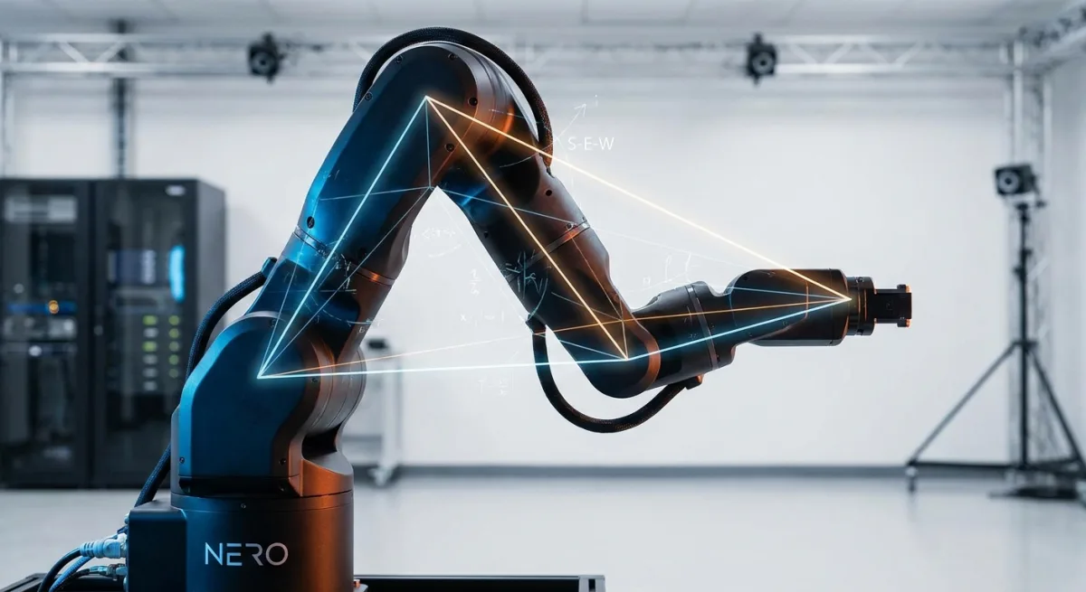
• The NERO 7-DoF robotic arm (Spherical Shoulder - Revolute Elbow - Spherical Wrist configuration).
• Basic understanding of transformation matrices and the S-E-W (Shoulder-Elbow-Wrist) geometric triangle.

1. Extract the shoulder (S), wrist (W), and elbow joint angle (θ4) from the target pose. This establishes the foundational geometry of the S-E-W triangle required for the closed-form solution, independent of the arm angle.

def _compute_swe_from_target(T07: np.ndarray, p: NeroParams) -> Tuple[np.ndarray, np.ndarray, Optional[float], np.ndarray]:
    R = T07[:3, :3]
    p_target = T07[:3, 3]
    z7 = R[:, 2]
    d6 = float(p.d_i[6])
    d1 = float(p.d_i[0])
    # End-effector flange center
    O7 = p_target - p.post_transform_d8 * z7
    # Wrist center W: offset backward from the flange by d6
    W = O7 - d6 * z7
    # Shoulder center S: fixed at height d1 above the base
    S = np.array([0.0, 0.0, d1], dtype=float)
    # Solve the absolute value of θ4 using the law of cosines
    q4_abs = _solve_theta4_from_triangle(S, W, p)
    # Unit vector from shoulder to wrist
    v_sw = W - S
    n_sw = np.linalg.norm(v_sw)
    u_sw = v_sw / n_sw if n_sw > 1e-12 else np.array([0.0, 0.0, 1.0])
    return S, W, q4_abs, u_sw

You will also need the helper function to solve the absolute value of the elbow joint angle using the law of cosines.

def _solve_theta4_from_triangle(S: np.ndarray, W: np.ndarray, p: NeroParams) -> Optional[float]:
    l_sw = np.linalg.norm(W - S)
    l_se = abs(p.d_i[2])
    l_ew = abs(p.d_i[4])
    c4 = (l_sw**2 - l_se**2 - l_ew**2) / (2.0 * l_se * l_ew)
    c4 = np.clip(c4, -1.0, 1.0)
    return math.acos(c4)

2. Compute the elbow point (E) using the arm angle (ψ). This step is the geometric core of the algorithm, projecting the circle center onto the SW line to find the exact elbow position in 3D space.

def _elbow_from_arm_angle(S: np.ndarray, W: np.ndarray, theta0: float, p: NeroParams) -> Optional[np.ndarray]:
    l_se = abs(p.d_i[2])
    l_ew = abs(p.d_i[4])
    sw = W - S
    l_sw = np.linalg.norm(sw)
    u_sw = sw / l_sw
    # Projection of circle center C onto line SW
    x = (l_se**2 - l_ew**2 + l_sw**2) / (2.0 * l_sw)
    r2 = l_se**2 - x**2
    r = math.sqrt(max(0.0, r2))
    C = S + x * u_sw
    # Construct circle-plane coordinate system e1, e2
    os_vec = S.copy()
    t = np.cross(os_vec, u_sw)
    e1 = t / np.linalg.norm(t)
    e2 = np.cross(u_sw, e1)
    e2 = e2 / np.linalg.norm(e2)
    # Compute elbow point E from arm angle theta0
    E = C + r * (math.cos(theta0) * e1 + math.sin(theta0) * e2)
    return E

3. Solve all joint angles analytically from the S-E-W triangle. This provides a direct closed-form solution for the shoulder joints (q1, q2, q3) and extracts the wrist joints (q5, q6, q7) directly from the transformation matrix.

def _solve_q123_from_swe(E: np.ndarray, W: np.ndarray, q4: float, p: NeroParams) -> List[np.ndarray]:
    d0 = p.d_i[0]
    d2 = p.d_i[2]
    d4 = p.d_i[4]
    Ex, Ey, Ez = E
    # q2
    c2 = (Ez - d0) / d2
    c2 = np.clip(c2, -1.0, 1.0)
    s2_abs = math.sqrt(max(0.0, 1.0 - c2**2))
    s4 = math.sin(q4)
    c4 = math.cos(q4)
    sols = []
    # Traverse both positive and negative s2 configurations
    for s2 in (s2_abs, -s2_abs):
        # q1
        c1 = -Ex / (d2 * s2)
        s1 = -Ey / (d2 * s2)
        n1 = math.hypot(c1, s1)
        c1 /= n1
        s1 /= n1
        q1 = math.atan2(s1, c1)
        q2 = math.atan2(s2, c2)
        # q3
        v = W - E
        col2 = -v / d4
        u1, u2, u3 = col2
        b1 = (s2 * c1 * c4 - u1) / s4
        b2 = (u2 - s1 * s2 * c4) / s4
        s3 = s1 * b1 + c1 * b2
        c2c3 = -c1 * b1 + s1 * b2
        c3 = c2c3 / c2 if abs(c2) > 1e-8 else (u3 + c2 * c4) / (s2 * s4)
        n3 = math.hypot(s3, c3)
        s3 /= n3
        c3 /= n3
        q3 = math.atan2(s3, c3)
        sols.append(np.array([q1, q2, q3]))
    return sols

Next, extract the wrist joint angles directly from the transformation matrix T47.

def _extract_567_from_T47_paper(T47: np.ndarray) -> List[np.ndarray]:
    sols = []
    c6 = np.clip(T47[1, 2], -1.0, 1.0)
    for sgn in (1.0, -1.0):
        s6 = sgn * math.sqrt(max(0.0, 1.0 - c6**2))
        if abs(s6) < 1e-8:
            continue
        th6 = math.atan2(s6, c6)
        th5 = math.atan2(T47[2, 2] / s6, T47[0, 2] / s6)
        th7 = math.atan2(T47[1, 1] / s6, -T47[1, 0] / s6)
        sols.append(np.array([th5, th6, th7]))
    return sols

4. Determine the feasible region of the arm angle to respect joint limits. This guarantees that all joints remain inside their physical limits by finding the intersection of all valid intervals.

def _get_theta0_feasible_region(T07: np.ndarray, p: NeroParams, step: float = 0.01) -> List[float]:
    feasible = []
    for theta0 in np.arange(-math.pi, math.pi, step):
        if _ik_one_arm_angle(T07, theta0, p):
            feasible.append(float(theta0))
    return feasible

5. Optimize the arm angle using a weighted quadratic objective function. This transforms the problem into a one-dimensional minimization, ensuring a globally optimal solution without local minima.

def _weight_limits(q: float, q_min: float, q_max: float) -> float:
    span = q_max - q_min
    x = 2.0 * (q - (q_min + q_max) * 0.5) / span
    a = 2.38
    b = 2.28
    if x >= 0:
        den = math.exp(a * (1 - x)) - 1
        return b * x / den
    else:
        den = math.exp(a * (1 + x)) - 1
        return -b * x / den

Apply the optimal arm-angle search strategy to find the best configuration.

def _optimal_theta0(feasible_theta0, T07, p, q_prev):
    best_cost = inf
    best_t = feasible_theta0[0]
    for t in feasible_theta0:
        sols = _ik_one_arm_angle(T07, t, p)
        for q_full in sols:
            q = q_full[:7]
            cost = 0
            for i in range(7):
                lo, hi = p.joint_limits[i]
                w = _weight_limits(q[i], lo, hi)
                dq = abs(q[i] - q_prev[i])
                cost += w * dq * dq
            if cost < best_cost:
                best_cost = cost
                best_t = t
    return best_t

6. Execute the solver in your ROS2 environment to generate null-space motion. This allows the robot to automatically perform self-reconfiguration while keeping the end-effector fixed.

import numpy as np
from ik_solver import ik_arm_angle, NeroParams

# Define target end-effector pose
T = np.eye(4)
T[:3, 3] = [0.5, 0.0, 0.5]

# Solve inverse kinematics
q_best, feasible_set = ik_arm_angle(T)
print("Optimal joint configuration:", q_best)
print("Number of feasible arm angles:", len(feasible_set))

The shift from numerical Jacobian solvers to a pure geometric closed-form solution marks a critical upgrade for embodied AI and edge robotics. Traditional iterative methods consume significant CPU cycles and are prone to oscillation when approaching singularities. By reducing the redundancy problem to a single 1D optimization over the arm angle, this solver guarantees real-time performance.

For developers building autonomous systems in ROS2, this efficiency translates directly into hardware capabilities. Freeing up computational overhead from the IK solver allows edge devices to allocate more processing power to complex vision models and dynamic path planning. Furthermore, the natural embedding of null-space motion ensures that 7-DoF arms can smoothly navigate confined spaces without the erratic joint snapping common in older numerical approaches.